Introduction – Why Does a Stationary Sensor Still Detect Motion?
Imagine an Inertial Navigation System (INS) installed in an aircraft, an autonomous vehicle, or a stabilized electro-optical system. The system relies on gyroscopes to measure angular velocity and accelerometers to measure acceleration.
Both types of sensors are essential components of an Inertial Measurement Unit (IMU), and their performance directly influences the quality of the information provided to the navigation or control system.
But what happens when these sensors are placed on a completely stationary surface?
Ideally, a gyroscope should report zero angular velocity because no rotation is taking place. An accelerometer, on the other hand, will still measure the effect of gravity, depending on its orientation.
In theory, as long as the sensors remain stationary, we might expect their outputs to remain perfectly constant.
In practice, they do not.
Even when a sensor is at rest, its measurements fluctuate slightly over time. Some fluctuations are small, rapid, and random, while others appear as slow, gradual changes in the sensor’s bias.
These effects do not necessarily indicate a malfunction. They are inherent characteristics of real-world sensors, particularly those based on Micro-Electro-Mechanical Systems (MEMS) technology.
The challenge arises when a navigation or control system interprets these measurement errors as actual motion.
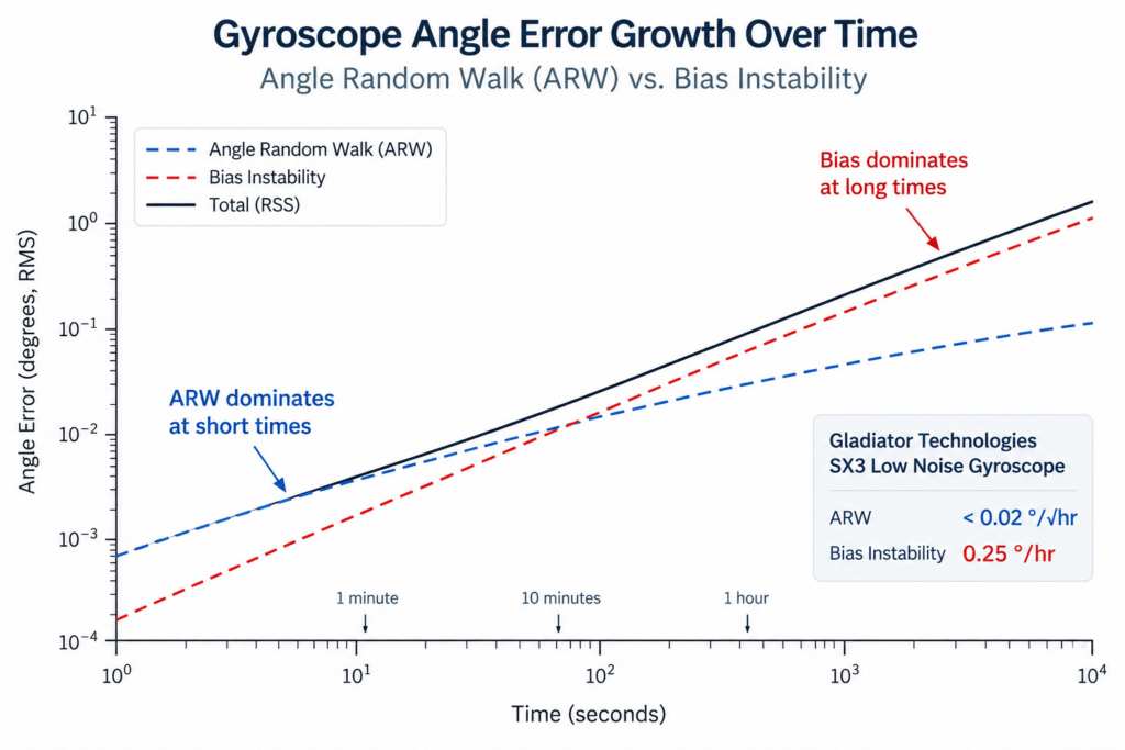
For example, noise in angular velocity measurements can accumulate into angular estimation errors, while errors in acceleration measurements can propagate into velocity and position errors.
The greater the required accuracy, or the longer a system must operate without external corrections, the more important it becomes to understand sensor noise and drift.
This is where Allan Deviation becomes particularly valuable.
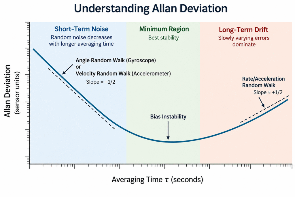
Allan Deviation is a statistical technique used to evaluate how measurement stability changes across different averaging times. It helps engineers identify and characterize different noise processes that affect inertial sensors.
In this article, we will explain the method, demonstrate how to interpret an Allan Deviation plot, and explore four important performance parameters:
- Angle Random Walk (ARW): Random noise in gyroscope measurements that contributes to accumulated angular uncertainty.
- Velocity Random Walk (VRW): Random noise in accelerometer measurements that contributes to accumulated velocity uncertainty.
- Bias Instability: Slow statistical fluctuations in a sensor’s measurement bias.
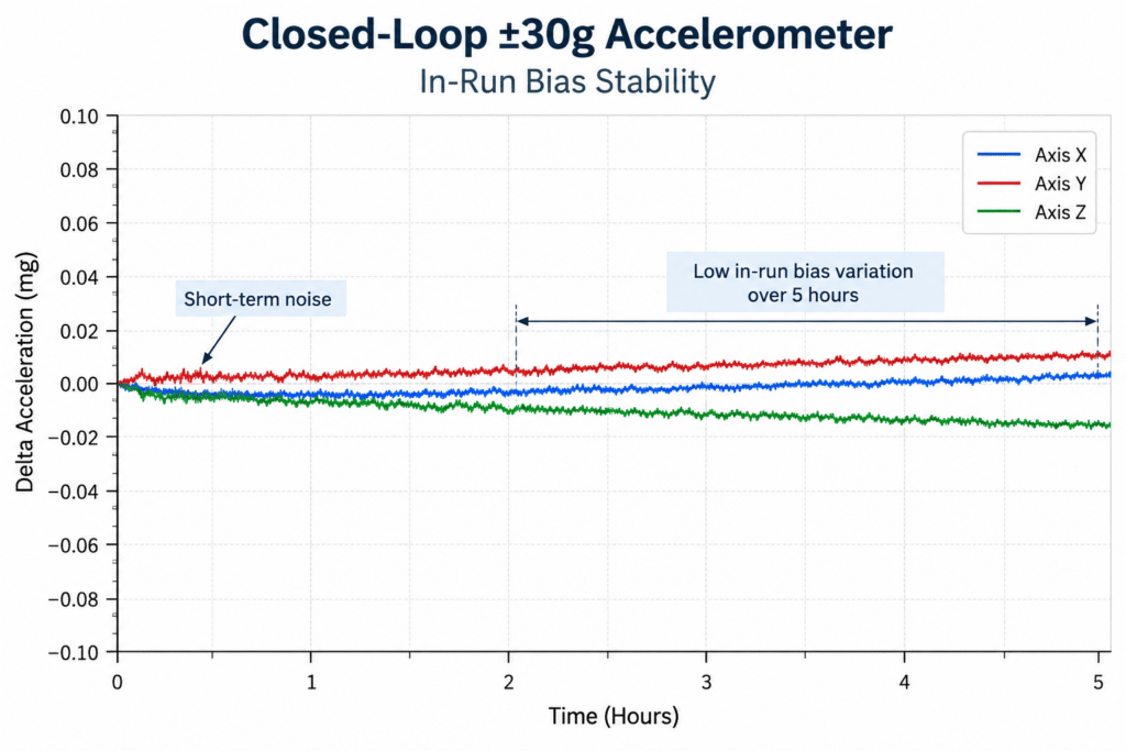
- In-Run Bias Stability: The stability of a sensor’s bias during continuous operation.
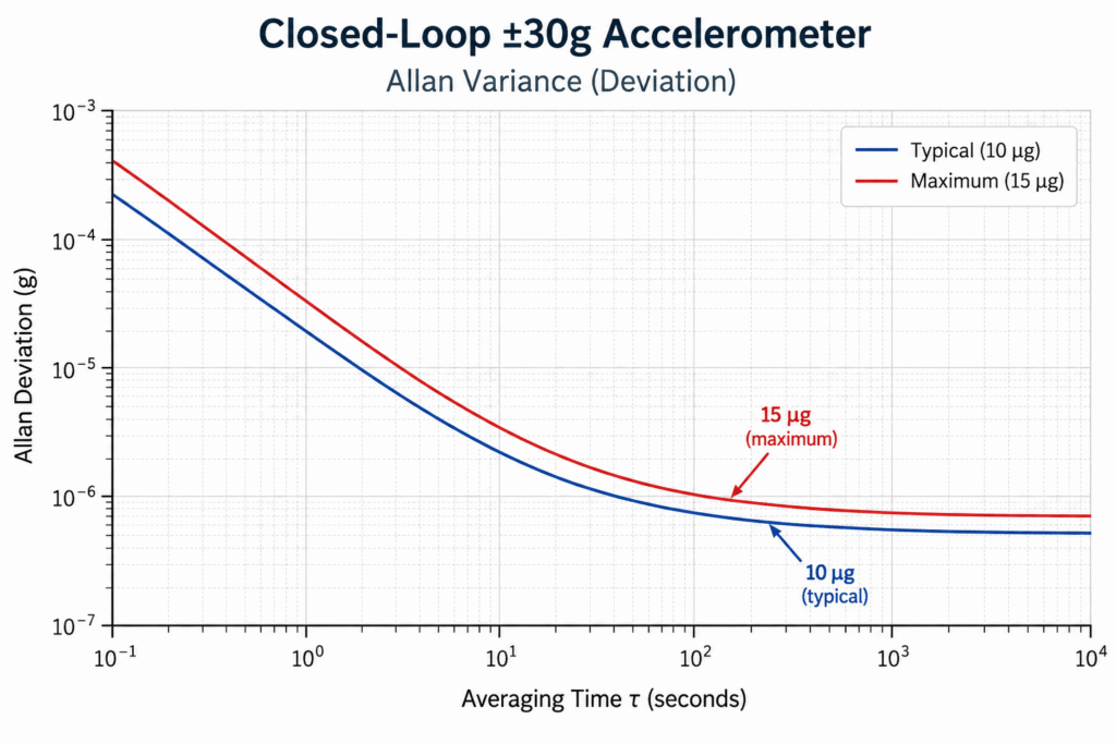
We will also examine measurement data presented by Gladiator Technologies for its closed-loop accelerometers and discuss the significance of low-noise performance in the company’s next-generation SX3 Low Noise inertial sensor technology.
1. What Is Allan Deviation? A Simple Explanation
Suppose we want to evaluate how stable a sensor’s measurements are over time.
We place the sensor in a stationary position, collect thousands of samples, and discover that the measured values fluctuate slightly from one sample to the next.
The intuitive solution is to calculate an average.
By averaging ten measurements, some of the random noise may cancel out. Averaging one hundred measurements may produce an even more stable result.
But does increasing the averaging time always improve measurement stability?
Not necessarily.
Over short time intervals, random noise may dominate the sensor output. Averaging helps reduce the influence of this noise.
However, over longer intervals, slower variations may become significant. These can result from internal sensor processes, temperature changes, or other low-frequency noise mechanisms.
Consequently, increasing the averaging time does not guarantee continuous improvement.
What Does Allan Deviation Actually Measure?
Instead of examining only how individual measurements differ from the overall mean, Allan Deviation analyzes differences between averages calculated over successive time intervals.
The basic process is straightforward:
- Collect a continuous sequence of sensor measurements under controlled conditions.
- Divide the measurements into consecutive intervals of equal duration.
- Calculate the average measurement within each interval.
- Evaluate the differences between averages of adjacent intervals.
- Repeat the calculation using different averaging times, such as 1 second, 10 seconds, 100 seconds, and longer.
The Allan Deviation is derived from the square root of half the mean squared difference between adjacent interval averages.
By repeating this process across multiple averaging times, engineers obtain a curve showing how sensor measurement stability changes with the observation timescale.
In simple terms, Allan Deviation reveals how different noise and drift mechanisms influence sensor stability over time.
An important distinction is that Allan Deviation does not directly measure a sensor’s absolute accuracy.
A sensor may exhibit exceptionally low Allan Deviation while still having a significant constant bias or calibration error.
For this reason, Allan Deviation should be used alongside other performance evaluations, including calibration accuracy, scale-factor errors, temperature sensitivity, and bias stability measurements.