flagעברית
flagEnglish
3 Rabinovich St., Petah-Tikva, Israel
+972 3 9047744
office@amironic.co.il
Facebook
Twitter
LinkedIn
YouTube
  • Products
    • MEMS Inertial
      • Gyros & Accels
      • IMU
      • Inertial Navigation
      • AHRS
    • Circuit Breakers
      • Airpax Circuit Breakers
      • Electronic Circuit Breakers
      • Aircraft Circuit Breakers
      • Thermal Circuit Breakers
      • Sealing Solutions & Guards
    • Footswitches
      • Pedals & Bellows
      • USB
      • Air Switches
      • Medical
      • Modular Bases System
      • Industrial
      • Foot Potentiometers
      • Wireless
    • Mechanical & Transmissions
      • Gears
      • Sealing Solutions
      • Gearboxes
      • Couplings
      • Shafts & Bearings
      • Fasteners
      • Mechanical & Springs
      • Linear Motion
      • Anti-Vibration
    • Sensors
      • Thermostats
      • Temperature
      • Position
      • Pressure
      • Speed
      • Level Sensor
      • Load Cells
      • Flex Sensors
      • Membrane Potentiometer
    • Motors
      • Geared DC
      • Brushless DC
      • Step Motors with Gearbox
      • Torque Motors & Brushless Servo
      • DC Motors
    • Electronics
      • Xenon & IR Lamps
      • Counters & Meters
      • Microelectronics Packaging
      • Waterproof Switches
      • Micro Switches
    • Hand Control
      • Operator Controls (JOYSTICK)
      • Electrical
      • Pneumatic (Medical)
      • USB Hand Control
      • Air Push Button
      • Pressure Switch
      • IR Switch
    • Power Solutions
      • Rugged & Military Power Supply
      • Input Power Protection
      • Sealed Military Power Adaptor
      • Triple Output Military Power Supply Series – up to 250 W
    • Materials
      • Molybdenum and Advanced Alloys (TZM, MOLA, HCT)
      • Tungsten (Wolfram) and Advanced Alloys – High-Performance Materials for Extreme Conditions
      • Materials for Gears
  • Shop
  • Companies
  • About Amironic
  • News
  • Contact
Product was added to your cart

Cart

waze

Allan Deviation in MEMS Sensors: Understanding Noise and Drift in Gyroscopes and Accelerometers

MEMS Inertial26/10/2026amironicLTD

Introduction – Why Does a Stationary Sensor Still Detect Motion?

Imagine an Inertial Navigation System (INS) installed in an aircraft, an autonomous vehicle, or a stabilized electro-optical system. The system relies on gyroscopes to measure angular velocity and accelerometers to measure acceleration.

Both types of sensors are essential components of an Inertial Measurement Unit (IMU), and their performance directly influences the quality of the information provided to the navigation or control system.

But what happens when these sensors are placed on a completely stationary surface?

Ideally, a gyroscope should report zero angular velocity because no rotation is taking place. An accelerometer, on the other hand, will still measure the effect of gravity, depending on its orientation.

In theory, as long as the sensors remain stationary, we might expect their outputs to remain perfectly constant.

In practice, they do not.

Even when a sensor is at rest, its measurements fluctuate slightly over time. Some fluctuations are small, rapid, and random, while others appear as slow, gradual changes in the sensor’s bias.

These effects do not necessarily indicate a malfunction. They are inherent characteristics of real-world sensors, particularly those based on Micro-Electro-Mechanical Systems (MEMS) technology.

The challenge arises when a navigation or control system interprets these measurement errors as actual motion.

For example, noise in angular velocity measurements can accumulate into angular estimation errors, while errors in acceleration measurements can propagate into velocity and position errors.

The greater the required accuracy, or the longer a system must operate without external corrections, the more important it becomes to understand sensor noise and drift.

This is where Allan Deviation becomes particularly valuable.

Allan Deviation is a statistical technique used to evaluate how measurement stability changes across different averaging times. It helps engineers identify and characterize different noise processes that affect inertial sensors.

In this article, we will explain the method, demonstrate how to interpret an Allan Deviation plot, and explore four important performance parameters:

  • Angle Random Walk (ARW): Random noise in gyroscope measurements that contributes to accumulated angular uncertainty.
  • Velocity Random Walk (VRW): Random noise in accelerometer measurements that contributes to accumulated velocity uncertainty.
  • Bias Instability: Slow statistical fluctuations in a sensor’s measurement bias.
  • In-Run Bias Stability: The stability of a sensor’s bias during continuous operation.

We will also examine measurement data presented by Gladiator Technologies for its closed-loop accelerometers and discuss the significance of low-noise performance in the company’s next-generation SX3 Low Noise inertial sensor technology.


1. What Is Allan Deviation? A Simple Explanation

Suppose we want to evaluate how stable a sensor’s measurements are over time.

We place the sensor in a stationary position, collect thousands of samples, and discover that the measured values fluctuate slightly from one sample to the next.

The intuitive solution is to calculate an average.

By averaging ten measurements, some of the random noise may cancel out. Averaging one hundred measurements may produce an even more stable result.

But does increasing the averaging time always improve measurement stability?

Not necessarily.

Over short time intervals, random noise may dominate the sensor output. Averaging helps reduce the influence of this noise.

However, over longer intervals, slower variations may become significant. These can result from internal sensor processes, temperature changes, or other low-frequency noise mechanisms.

Consequently, increasing the averaging time does not guarantee continuous improvement.

What Does Allan Deviation Actually Measure?

Instead of examining only how individual measurements differ from the overall mean, Allan Deviation analyzes differences between averages calculated over successive time intervals.

The basic process is straightforward:

  1. Collect a continuous sequence of sensor measurements under controlled conditions.
  2. Divide the measurements into consecutive intervals of equal duration.
  3. Calculate the average measurement within each interval.
  4. Evaluate the differences between averages of adjacent intervals.
  5. Repeat the calculation using different averaging times, such as 1 second, 10 seconds, 100 seconds, and longer.

The Allan Deviation is derived from the square root of half the mean squared difference between adjacent interval averages.

By repeating this process across multiple averaging times, engineers obtain a curve showing how sensor measurement stability changes with the observation timescale.

In simple terms, Allan Deviation reveals how different noise and drift mechanisms influence sensor stability over time.

An important distinction is that Allan Deviation does not directly measure a sensor’s absolute accuracy.

A sensor may exhibit exceptionally low Allan Deviation while still having a significant constant bias or calibration error.

For this reason, Allan Deviation should be used alongside other performance evaluations, including calibration accuracy, scale-factor errors, temperature sensitivity, and bias stability measurements.
2. How to Read an Allan Deviation Plot

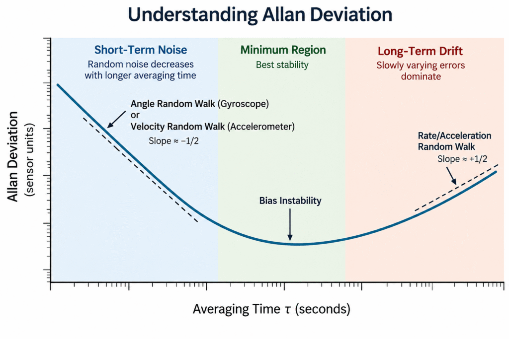
Now that we understand the basic principle, let’s examine the first Allan Deviation plot.

The graph illustrates how measurement stability changes as the averaging time increases. The same principles apply to both gyroscopes and accelerometers, although their physical measurement units differ.

Important: This is a conceptual illustration, not actual measurement data from a specific sensor.

Horizontal Axis – Averaging Time

The horizontal axis represents the averaging time, commonly denoted by the Greek letter τ (tau).

For example, when the averaging time is one second, the sensor data is divided into one-second intervals, and the average measurement is calculated for each interval.

When the averaging time increases to 100 seconds, the same calculation is performed using longer intervals.

This allows engineers to determine whether longer averaging periods improve measurement stability or whether slower noise processes and drift begin to dominate.

Vertical Axis – Allan Deviation

The vertical axis represents Allan Deviation, a statistical measure derived from the differences between the averages of adjacent measurement intervals.

A lower Allan Deviation value indicates greater measurement stability over the specified averaging time.

For a gyroscope measuring angular velocity, Allan Deviation may be expressed in degrees per second (°/s). For an accelerometer, it may be expressed in acceleration units such as mg or µg.

Both axes are typically displayed on logarithmic scales, allowing engineers to examine sensor behavior across a wide range of averaging times and noise levels.

The Three Main Regions of an Allan Deviation Plot

Region 1 – Short-Term Noise

On the left side of the plot, the Allan Deviation curve generally decreases as the averaging time increases.

In this region, high-frequency random noise often dominates the measurement. Averaging reduces the influence of this noise.

When white noise is the dominant mechanism, the curve exhibits an approximate slope of -1/2 on a logarithmic plot.

For gyroscopes, this region is associated with Angle Random Walk (ARW). For accelerometers, the corresponding noise parameter is Velocity Random Walk (VRW).

Region 2 – Minimum Region

As the averaging time increases, the downward slope gradually becomes less pronounced. The curve may approach a nearly horizontal region or reach a minimum.

At this stage, the influence of high-frequency white noise has decreased, while slower noise processes become more significant.

One important mechanism is Bias Instability, which describes slow statistical fluctuations in the sensor’s measurement bias.

This region is particularly valuable when evaluating sensor stability over extended periods.

However, the minimum point of an Allan Deviation curve does not necessarily represent pure Bias Instability. Accurate identification requires examining the curve’s slope, shape, and underlying noise mechanisms.

Region 3 – Long-Term Drift

On the right side of the plot, the Allan Deviation curve may begin to rise.

This indicates that increasing the averaging time no longer improves measurement stability.

At longer timescales, slow noise processes may dominate. In gyroscopes, these can include Rate Random Walk, while accelerometers may exhibit analogous low-frequency noise behavior.

Environmental influences, particularly temperature variations, can also contribute to long-term changes in sensor output.

It is therefore important to distinguish between the sensor’s intrinsic stochastic noise and environmental effects that may not have been fully controlled during testing.

The key takeaway: There is no single optimal averaging time for every sensor or application. An Allan Deviation plot helps engineers understand how measurement stability evolves over time and identify the dominant noise mechanisms at different timescales.


3. What Is Angle Random Walk (ARW) in a Gyroscope?

A gyroscope measures angular velocity, describing how quickly an object rotates around a particular axis.

To determine the angular displacement of an object, the measured angular velocity is integrated over time.

However, the gyroscope output also contains random noise.

Even when the sensor is completely stationary, integrating this noise introduces uncertainty into the calculated angle.

This effect is known as Angle Random Walk (ARW).

Imagine someone attempting to walk in a straight line while taking small, random steps to the left or right. Although these deviations have no consistent direction, the accumulated displacement from the intended path can increase over time.

Similarly, random noise in angular velocity measurements produces growing uncertainty in the estimated angular position.

How Should ARW Be Interpreted?

ARW is commonly expressed in degrees per square root of hour (°/√hr).

A lower ARW value indicates a smaller contribution from white noise to the accumulated angular uncertainty.

For example, consider a gyroscope with an ARW of 0.02°/√hr.

Assuming ideal white noise, the approximate RMS angular uncertainty caused by this noise component alone is:

Integration Time Approximate RMS Angular Error
1 minute 0.0026°
10 minutes 0.0082°
1 hour 0.0200°

These values are calculated theoretical examples, not experimental measurements.

They follow the relationship:

RMS Angular Error ≈ ARW × √Time

where time is expressed in hours when ARW is specified in °/√hr.

The calculation considers only the white-noise component represented by ARW. It excludes bias errors, temperature effects, calibration errors, and other sources of measurement uncertainty.

SX3 Low Noise – Why Does This Matter?

Gladiator Technologies has presented an ARW value below 0.02°/√hr for its next-generation SX3 Low Noise sensor technology.

This indicates a low level of angular random noise under the reported measurement conditions.

Such performance can be particularly valuable in applications requiring precise motion sensing, including electro-optical stabilization, inertial navigation, and advanced motion control systems.

However, ARW alone does not determine the overall accuracy of an inertial system.

Bias stability, sensor bandwidth, measurement latency, environmental conditions, and system-level calibration also influence actual performance.

Furthermore, technology-level measurement results should not automatically be interpreted as guaranteed specifications for every SX3-based product configuration.


4. What Is Velocity Random Walk (VRW) in an Accelerometer?

Accelerometers exhibit a similar noise-related phenomenon, but instead of accumulated angular uncertainty, the result is accumulated velocity uncertainty.

An accelerometer measures acceleration. When an inertial navigation system needs to estimate velocity, it integrates the acceleration measurements over time.

However, accelerometer output also contains random noise.

When this noise is integrated, it introduces uncertainty into the calculated velocity. For white acceleration noise, the RMS velocity uncertainty increases approximately with the square root of the integration time.

This phenomenon is known as Velocity Random Walk (VRW).

The fundamental difference between ARW and VRW lies in the physical quantity affected by the accumulated measurement noise.

Parameter Gyroscope Accelerometer
Measured quantity Angular velocity Acceleration
Random walk parameter ARW VRW
Quantity obtained through integration Angle Velocity
Accumulated uncertainty Angular uncertainty Velocity uncertainty

In an inertial navigation system, velocity estimation errors can subsequently contribute to position errors when acceleration measurements are integrated a second time.

This is one reason why accelerometer noise performance is just as important as gyroscope noise performance in high-accuracy inertial navigation applications.

Why Does VRW Matter When Comparing Accelerometers?

Two accelerometers may offer the same measurement range, such as ±30g, while exhibiting significantly different noise characteristics.

An accelerometer with lower VRW generally contributes less white-noise-induced uncertainty to the estimated velocity, assuming comparable measurement conditions and other sensor characteristics.

However, VRW alone does not provide a complete picture of accelerometer performance.

To evaluate long-term measurement stability, engineers must also examine bias stability, temperature sensitivity, and Allan Deviation results.

An important distinction when comparing datasheets: Accelerometer manufacturers may express random noise performance using different units.

Acceleration noise density is commonly specified in µg/√Hz, whereas VRW can also be expressed in velocity-per-square-root-of-time units, such as m/s/√hr.

These quantities are related through the integration of acceleration noise, but their numerical values should not be compared directly without accounting for the units and the manufacturer’s definitions.

This distinction becomes particularly important when evaluating closed-loop accelerometers from different manufacturers.

5. From Theory to Real-World Performance – Gladiator Technologies Accelerometers

So far, we have explored the principles of Allan Deviation and the significance of random noise in gyroscopes and accelerometers.

Now, let’s examine how these parameters relate to the performance of real-world inertial sensors.

Gladiator Technologies develops advanced inertial sensing solutions, including gyroscopes, accelerometers, and Inertial Measurement Units (IMUs), for applications requiring low noise, high stability, and reliable performance under demanding environmental conditions.

Among its product families are closed-loop accelerometers, which use a feedback mechanism to apply a balancing force to the internal proof mass in response to external acceleration.

This force-rebalance approach can provide excellent measurement stability and support improved sensor performance, depending on the specific design and implementation.

Allan Deviation Measurements of a ±30g Closed-Loop Accelerometer

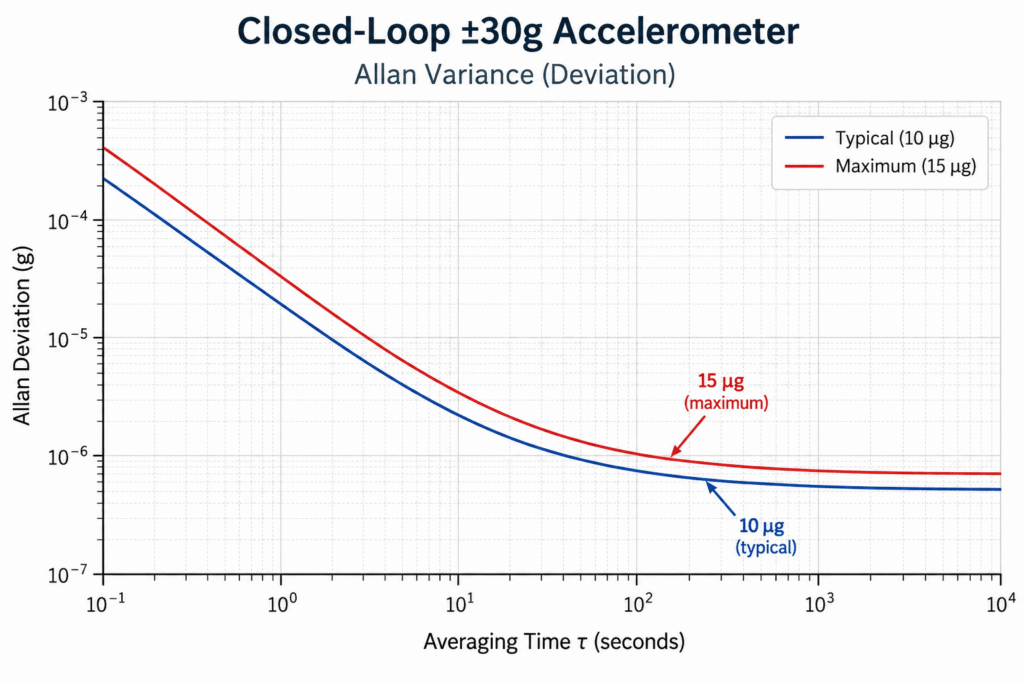
In its technical presentation, Gladiator Technologies provides Allan Deviation measurement results for a closed-loop accelerometer with a ±30g measurement range.

The graph shows Allan Deviation decreasing as the averaging time increases, followed by a region where the curve begins to flatten.

For the stability characteristic highlighted in this measurement, the manufacturer reports:

  • Typical: 10 µg – Typical reported value.
  • Maximum: 15 µg – Maximum value indicated in the presented data.

To put these figures into perspective, 10 micro-g corresponds to just 0.00001g, or approximately 0.000098 m/s².

This is an extremely small acceleration level, illustrating the measurement sensitivity and stability required in high-performance inertial sensing applications.

However, this value should not be interpreted as a guarantee that the accelerometer provides an absolute accuracy of 10 µg under all operating conditions.

It represents a stability characteristic derived from the manufacturer’s reported measurements, not a comprehensive specification of total measurement error.

GA100, GA200, and GA300 Closed-Loop Accelerometer Families

Gladiator Technologies offers three families of single-axis closed-loop accelerometers designed for different acceleration measurement ranges.

Accelerometer Family Measurement Range VRW / Acceleration Noise Density (D Version) Bandwidth
GA100 ±15g 20 µg/√Hz >300 Hz
GA200 ±30g 20 µg/√Hz >300 Hz
GA300 ±70g 20 µg/√Hz >300 Hz

These figures refer to the D versions and are based on preliminary performance specifications published by Gladiator Technologies.

Technical note: The manufacturer identifies the 20 µg/√Hz parameter as VRW. These units are also commonly used to express acceleration noise density. When comparing accelerometers from different manufacturers, engineers should verify the definitions, measurement conditions, and units used in each datasheet.

Another important distinction concerns the stability specifications.

For the D versions, Gladiator Technologies lists the following In-Run / Short-Term (5hr) Stability values:

Accelerometer Family In-Run Stability Short-Term Stability (5 hr)
GA100 7 µg 60 µg
GA200 7 µg 60 µg
GA300 16 µg 125 µg

These values represent different stability characteristics as defined in the manufacturer’s preliminary specifications. They should not be interpreted as interchangeable measurements or as guarantees of total sensor accuracy.

The differences between these accelerometer families demonstrate why selecting an inertial sensor should involve more than simply choosing the highest available measurement range.

For example, a system designed to measure accelerations up to ±15g does not necessarily require an accelerometer capable of measuring ±70g.

Engineers must also consider noise performance, bias stability, vibration conditions, bandwidth, and the overall requirements of the application.

The engineering advantage lies in selecting an accelerometer that matches the application’s motion profile and accuracy requirements, rather than relying solely on maximum acceleration range.


6. What Is Bias Instability, and Why Does It Matter?

Until now, we have focused primarily on random noise, whose influence can often be reduced through averaging.

However, inertial sensors face another challenge that can be equally important, or even more significant in certain applications:

The sensor’s measurement bias does not necessarily remain constant over time.

This behavior is closely related to Bias Instability.

First, What Is Sensor Bias?

Consider a gyroscope resting on a stationary surface.

Ideally, its output should indicate an angular velocity of zero degrees per second.

However, suppose the sensor consistently reports 0.01°/s even though no rotation is occurring.

This represents a measurement bias of 0.01°/s.

If the bias were perfectly constant, it could be measured and compensated for through calibration.

In practice, however, sensor bias may change during operation.

For example, the gyroscope may initially report a bias of 0.01°/s, but this value may gradually fluctuate even while the sensor remains stationary.

These slow variations make it more difficult for the navigation or control system to distinguish actual motion from changes originating within the sensor itself.

Bias Instability vs. In-Run Bias Stability

Both terms describe aspects of measurement bias stability, but they do not necessarily represent the same performance parameter.

Bias Instability is a statistical measure associated with slow fluctuations in sensor bias, commonly characterized through Allan Deviation analysis.

In particular, it is often associated with low-frequency flicker noise, although the extraction method depends on the noise model and analysis procedure.

In-Run Bias Stability, on the other hand, describes the stability of sensor bias during continuous operation.

Its exact definition and calculation method may vary between manufacturers and datasheets. Depending on the specification, it may be derived from statistical analysis, direct measurements over a defined operating period, or other test procedures.

Therefore, when comparing inertial sensors, it is essential to confirm that the reported values are based on comparable definitions, measurement methods, and test conditions.

Why Can a Small Bias Cause a Large Navigation Error?

Consider a gyroscope with a constant, uncompensated bias of 0.01°/s.

If an inertial navigation system integrates this angular velocity error over one minute, the resulting angular error will be:

0.01°/s × 60 s = 0.6°

After ten minutes, the accumulated angular error will reach:

0.01°/s × 600 s = 6°

This example illustrates the accumulation of angular error caused by a constant, uncompensated bias.

It is not a calculation of Bias Instability.

The distinction is important because Bias Instability describes stochastic fluctuations in bias, rather than a fixed offset that produces a predictable linear drift.

Nevertheless, the example demonstrates why even small bias errors can become significant in inertial navigation systems operating without continuous external corrections.

SX3 Low Noise – Combining Low Random Noise with Improved Bias Stability

For its next-generation SX3 Low Noise technology, Gladiator Technologies has presented a best-case measured Bias Instability value of 0.25°/hr, together with an Angle Random Walk value below 0.02°/√hr.

These reported results highlight two important performance objectives:

  • Reducing high-frequency random noise in angular velocity measurements.
  • Improving the stability of the sensor’s measurement bias over time.

Together, these characteristics can help reduce uncertainty in inertial measurements, particularly in applications where accurate angular information is required over extended operating periods.

However, it is important to distinguish between Bias Instability, expressed in degrees per hour, and accumulated angular error.

A Bias Instability value of 0.25°/hr does not necessarily mean that the angular error will be 0.25° after one hour.

The actual error depends on the underlying noise processes, operating conditions, integration time, and the correction methods implemented by the navigation system.

Furthermore, the reported SX3 values represent performance results presented for the technology and should not automatically be treated as guaranteed specifications for every product configuration.

In advanced inertial navigation and stabilization systems, low ARW and improved bias stability can contribute to more accurate motion estimation, especially when combined with appropriate control-system design, signal processing, temperature compensation, and sensor calibration.

7. In-Run Bias Stability – What Happens After Several Hours of Operation?

We have already explored how Allan Deviation helps identify different noise characteristics and how Bias Instability describes slow statistical fluctuations in sensor bias.

However, from an engineering perspective, it is equally important to understand how an inertial sensor behaves during continuous operation.

Consider an accelerometer installed in an Inertial Navigation System (INS) operating for several hours.

Even if the sensor remains stationary, its output may gradually change over time.

Such changes can result from internal stabilization processes, temperature variations, or low-frequency noise mechanisms.

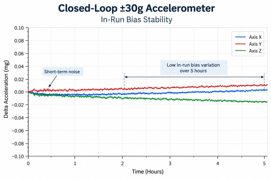
One way to evaluate this behavior is through In-Run Bias Stability measurements.

How to Interpret an In-Run Bias Stability Plot

Unlike an Allan Deviation plot, which shows a statistical stability measure as a function of averaging time, a time-history plot used to assess In-Run Bias Stability shows how the sensor output evolves during the actual test period.

Two important characteristics can often be observed:

1. Short-Term Fluctuations Around the Measured Value

These fluctuations may be associated with short-term measurement noise.

They appear as rapid, relatively small variations in the sensor output, giving the measurement curve a slightly irregular appearance.

2. Gradual Changes in the Measured Value

When the measurement curve gradually shifts upward or downward, this may indicate a change in the sensor’s bias over time.

Such behavior can result from temperature effects, internal stabilization, or other slow processes.

Both characteristics matter, but they affect the system differently.

High-frequency noise may influence signal quality and control-system performance, while slow bias variations can contribute to accumulated errors in systems that integrate inertial measurements over time.

A time-history plot helps visualize these effects, although a numerical In-Run Bias Stability specification must still be interpreted according to the manufacturer’s defined calculation method.

Stability During Continuous Operation – Gladiator Technologies Accelerometers

In measurements presented by Gladiator Technologies for a ±30g closed-loop accelerometer, the acceleration output can be observed over a test period lasting several hours.

The measurement curves show relatively small fluctuations, together with gradual changes in the measured acceleration.

These results illustrate why evaluating sensor stability over time is important, rather than focusing exclusively on instantaneous noise levels.

According to the preliminary performance specifications for the GA200-030-100D accelerometer, Gladiator Technologies reports:

  • In-Run Stability: 7 µg
  • Short-Term Stability (5 hr): 60 µg

These are two distinct stability parameters presented by the manufacturer.

They should not be treated as interchangeable values, and neither should be interpreted independently as a guarantee of total accelerometer accuracy.

For inertial navigation applications, the significance of these measurements depends on the manufacturer’s test methodology, environmental conditions, and the way sensor errors propagate through the navigation system.


8. How to Compare Gyroscopes and Accelerometers Correctly

One of the most common mistakes when selecting an inertial sensor is focusing on a single performance specification.

For example, two gyroscopes may offer the same angular rate measurement range while exhibiting significant differences in noise, bias stability, bandwidth, and latency.

Similarly, two accelerometers with identical ±30g measurement ranges may be suitable for entirely different applications.

A meaningful engineering comparison must therefore consider several performance characteristics together.

1. Random Noise – ARW and VRW

For gyroscopes, a lower Angle Random Walk (ARW) value indicates a smaller contribution from white noise to accumulated angular uncertainty.

For accelerometers, a lower Velocity Random Walk (VRW) value indicates a smaller contribution from white acceleration noise to accumulated velocity uncertainty.

However, comparisons must be performed using consistent definitions and units.

Manufacturers may express gyroscope and accelerometer noise performance differently, so values should be converted to equivalent units before drawing conclusions.

2. Bias Instability

A lower Bias Instability value may indicate better long-term bias stability over the relevant observation timescales.

However, the reported values must be interpreted carefully.

Different manufacturers may use different measurement procedures, estimation methods, and environmental conditions.

For a meaningful comparison, engineers should verify that the underlying definitions and test methods are compatible.

3. In-Run Bias Stability

In-Run Bias Stability is particularly important in systems operating continuously for extended periods.

When comparing specifications, engineers should examine:

  • The duration of the measurement.
  • Temperature conditions and thermal stabilization.
  • The statistical method used to calculate the reported value.
  • Whether the specification represents typical performance, a measured result, or a guaranteed maximum.

A single stability figure without its measurement context may provide an incomplete picture of real-world performance.

4. Bandwidth and Measurement Latency

Low noise does not automatically guarantee good performance in a high-speed control system.

Electro-optical stabilization systems, for example, may require both high sensor bandwidth and low measurement latency.

Aggressive digital filtering can reduce measurement noise, but it may also introduce additional delay and affect the dynamic response of the control loop.

Therefore, noise performance must be evaluated alongside bandwidth, latency, and the overall dynamic requirements of the application.

5. Environmental Conditions

Allan Deviation measurements are generally performed under controlled conditions.

In real-world applications, however, inertial sensors may be exposed to vibration, mechanical shock, temperature variations, and other environmental disturbances.

Sensor performance under these conditions may differ significantly from its behavior during a stationary laboratory measurement.

For this reason, Allan Deviation analysis does not replace environmental qualification testing or system-level performance evaluation.

Practical Example – Selecting an Inertial Sensor for Different Applications

Consider two systems with very different performance requirements.

Application 1 – Electro-Optical Camera Stabilization

An electro-optical stabilization system must detect rapid angular motion and respond with minimal delay.

In this application, important sensor characteristics include:

  • Low gyroscope noise.
  • Sufficient measurement bandwidth.
  • Low latency.
  • Appropriate dynamic response for the stabilization control loop.

Although bias stability remains relevant, fast and accurate motion detection may be a particularly important design priority.

Application 2 – Inertial Navigation Without Continuous External Corrections

An inertial navigation system estimates motion by integrating gyroscope and accelerometer measurements over time.

When external position or attitude corrections are unavailable for extended periods, sensor errors can accumulate.

In this application, both random noise and bias stability become critical factors affecting navigation accuracy.

Long-term bias behavior may have a particularly significant influence on accumulated navigation errors.

Both applications rely on inertial sensors, but their performance priorities are not necessarily the same.

The best sensor is not always the one with the lowest noise figure. It is the sensor whose overall performance characteristics best match the requirements of the application.

SX3 Low Noise – Combining Low Noise with High Bias Stability

Gladiator Technologies has presented the following performance results for its next-generation SX3 Low Noise inertial sensor technology:

  • Angle Random Walk (ARW): Below 0.02°/√hr
  • Bias Instability: 0.25°/hr in the best reported measurement

These results highlight the company’s focus on reducing random noise while improving bias stability.

For engineers developing advanced navigation, stabilization, and motion-control systems, both characteristics are important.

However, they must be evaluated alongside other essential parameters, including sensor bandwidth, latency, environmental performance, and application-specific requirements.

It is also important to distinguish between technology-level measurement results and guaranteed product specifications.

The reported SX3 performance values should not be interpreted as a guarantee of identical performance across all operating conditions or product configurations.

Final sensor selection should always be based on the latest manufacturer specifications for the specific product and configuration under consideration.

9. ARW vs. Bias Instability – Two Complementary Performance Parameters

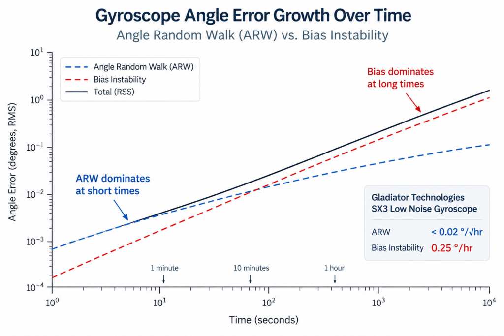
The fourth graph illustrates two different error mechanisms that can influence the angular position estimated from gyroscope measurements over time.

The blue curve represents the effect of Angle Random Walk (ARW), while the red curve conceptually illustrates the possible influence of slow bias-related errors.

The black curve demonstrates a possible mathematical combination of two independent error contributions.

It is important to emphasize that this is a conceptual illustration, not actual measurement data from a specific sensor or a prediction of SX3 navigation performance.

In particular, the red curve should not be interpreted as a direct mathematical representation of Bias Instability. Actual bias-related drift depends on the underlying stochastic processes and cannot generally be described by a single deterministic curve.

Why Is ARW Important?

When white noise in gyroscope measurements is integrated to calculate angular position, the accumulated RMS angular uncertainty increases approximately with the square root of time.

Therefore, a lower ARW value means a smaller contribution from random noise to the accumulated angular error.

This characteristic is particularly important in stabilization systems, electro-optical platforms, and applications requiring precise motion measurements.

Why Is Bias Instability Important?

Unlike high-frequency random noise, Bias Instability describes slow statistical fluctuations in the sensor’s measurement bias.

These fluctuations can affect the integration of angular velocity measurements and contribute to accumulated errors, especially in inertial navigation systems operating for extended periods without external corrections.

However, unlike a constant bias, the angular error associated with Bias Instability cannot be calculated simply by multiplying the reported Bias Instability value by the operating time.

The actual effect depends on the statistical behavior of the noise, the measurement duration, and the methods used by the navigation system to estimate and compensate for sensor errors.

What Does This Mean for SX3 Low Noise?

Gladiator Technologies has presented two notable performance results for its next-generation SX3 Low Noise technology:

  • Angle Random Walk (ARW): Below 0.02°/√hr
  • Bias Instability: 0.25°/hr in the best reported measurement

These results indicate low angular random noise and high bias stability under the relevant measurement conditions.

The combination is important because reducing high-frequency noise alone is not sufficient for advanced inertial systems. Engineers must also consider the slower error mechanisms that influence measurement stability over time.

When selecting a gyroscope or IMU, both ARW and Bias Instability should therefore be evaluated alongside bandwidth, latency, temperature stability, and application-specific requirements.


10. Selecting an Inertial Sensor – From Laboratory Measurements to Real-World Applications

Allan Deviation provides valuable insight into the noise and stability characteristics of inertial sensors.

However, selecting a sensor for a real-world system requires a broader engineering perspective.

Gladiator Technologies offers a range of inertial sensing solutions, from standalone gyroscopes and accelerometers to integrated Inertial Measurement Units (IMUs).

Its product portfolio includes:

GA100, GA200, and GA300 – Single-axis closed-loop accelerometer families with measurement ranges of ±15g, ±30g, and ±70g, respectively.

G300D and G400D – Digital gyroscope families designed for integration into motion measurement and control systems.

LMRK005, LMRK007, and LMRK008 – Inertial Measurement Unit families that integrate motion sensors within a compact assembly, depending on the specific product configuration.

SX3 Low Noise – A next-generation inertial sensing technology focused on improving noise performance and measurement stability.

Selecting the appropriate solution depends on several application requirements, including measurement range, bandwidth, operating duration, vibration and shock conditions, size and weight constraints, and communication interfaces.

For example, an electro-optical stabilization system may prioritize low gyroscope noise, high bandwidth, and minimal measurement latency.

An inertial navigation system, on the other hand, may place greater emphasis on bias stability and accumulated measurement errors over extended operating periods.

The best sensor is not necessarily the one with the most impressive individual specification, but the one that provides the most suitable balance of performance characteristics for the intended application.


11. Conclusion – What Can Allan Deviation Really Tell Us?

Allan Deviation is one of the most valuable statistical techniques for analyzing noise and stability in inertial sensors.

Unlike conventional standard deviation alone, Allan Deviation reveals how measurement stability changes with averaging time.

By analyzing the shape and slopes of an Allan Deviation curve, engineers can identify different noise mechanisms, estimate parameters such as ARW, VRW, and Bias Instability, and better understand sensor behavior across different timescales.

In gyroscopes, random noise contributes to uncertainty in the calculated angular position. In accelerometers, similar noise processes contribute to velocity uncertainty and, through further integration, position estimation errors.

The measurement data presented by Gladiator Technologies demonstrates how these analysis methods can be applied to characterize advanced closed-loop accelerometers.

Meanwhile, the reported SX3 Low Noise results highlight the importance of combining low angular noise with improved bias stability.

For engineers developing navigation, stabilization, and motion-control systems, understanding these parameters enables more meaningful sensor comparisons and better-informed design decisions.

Advanced Inertial Sensing Solutions from Gladiator Technologies

Amironic Ltd. represents Gladiator Technologies in Israel, providing advanced inertial sensing solutions for industrial, defense, and high-technology applications.

The available solutions include gyroscopes, accelerometers, and IMUs, with options to select configurations that meet specific application requirements.

Amironic’s engineering and technical sales team assists customers in evaluating sensor specifications, comparing performance characteristics, and selecting suitable inertial sensing solutions.

For additional information about SX3 Low Noise technology, GA100/GA200/GA300 closed-loop accelerometers, and Gladiator Technologies IMU solutions, contact the Amironic team.


Frequently Asked Questions (FAQ)

What Is Allan Deviation in MEMS Sensors?

Allan Deviation is a statistical method used to evaluate measurement stability as a function of averaging time. It helps identify and characterize different noise mechanisms in MEMS sensors, including white noise, Bias Instability, and slow drift-related processes.

What Is the Difference Between Allan Variance and Allan Deviation?

Allan Variance is calculated from the mean squared differences between averages of adjacent measurement intervals, divided by two. Allan Deviation is the square root of Allan Variance.

As a result, Allan Deviation is expressed in the same physical units as the measured quantity, while Allan Variance is expressed in squared units.

What Is ARW in a Gyroscope?

Angle Random Walk (ARW) is a measure of random noise in gyroscope angular velocity measurements and its contribution to accumulated angular uncertainty after integration.

A lower ARW value indicates a smaller contribution from white noise to the estimated angular position error.

What Is VRW in an Accelerometer?

Velocity Random Walk (VRW) describes the contribution of random acceleration noise to uncertainty in the calculated velocity after integrating accelerometer measurements over time.

Manufacturers may express related accelerometer noise specifications in different units, so consistent definitions are essential when comparing products.

What Is Bias Instability?

Bias Instability is a statistical measure associated with slow fluctuations in a sensor’s measurement bias.

It is commonly estimated using Allan Deviation analysis, depending on the assumed noise model and the calculation method.

Does Lower Allan Deviation Always Mean a More Accurate Sensor?

Not necessarily.

Allan Deviation characterizes measurement noise and stability, but it does not account for every source of sensor error.

Calibration errors, scale-factor errors, temperature sensitivity, vibration effects, and other characteristics must also be considered.

Can ARW and VRW Be Compared Directly?

No.

ARW relates to gyroscope noise and its effect on angular uncertainty, while VRW relates to accelerometer noise and its effect on velocity uncertainty.

They describe different physical quantities and cannot be compared directly as equivalent performance measures.

What Are the Reported Performance Figures for Gladiator Technologies SX3 Low Noise?

For its SX3 Low Noise technology, Gladiator Technologies has presented an Angle Random Walk value below 0.02°/√hr and a best-case measured Bias Instability value of 0.25°/hr.

These are reported technology-level performance results. Engineers should consult the latest manufacturer specifications for the relevant product configuration before integrating it into a system.


Technical Glossary

MEMS – Micro-Electro-Mechanical Systems: A technology used to manufacture miniature mechanical and electronic structures, including those used in gyroscopes and accelerometers.

IMU – Inertial Measurement Unit: A device that typically combines gyroscopes and accelerometers to measure motion and orientation-related quantities.

INS – Inertial Navigation System: A navigation system that uses inertial measurements to estimate motion, velocity, orientation, and position.

Allan Deviation: A statistical measure of measurement stability as a function of averaging time.

Allan Variance: The statistical variance measure from which Allan Deviation is calculated.

ARW – Angle Random Walk: A gyroscope noise parameter describing the contribution of random angular velocity noise to accumulated angular uncertainty.

VRW – Velocity Random Walk: An accelerometer noise parameter describing the contribution of random acceleration noise to accumulated velocity uncertainty.

Bias: A systematic measurement offset between the sensor output and the true value of the measured quantity.

Bias Instability: A statistical characteristic associated with slow fluctuations in sensor bias, commonly estimated using Allan Deviation analysis.

In-Run Bias Stability: A measure of sensor bias stability during continuous operation, as defined by the manufacturer’s test methodology.

Scale Factor: The relationship between a physical input quantity and the corresponding sensor output.

Closed-Loop Accelerometer: An accelerometer that uses a feedback mechanism to apply a balancing force to its internal proof mass.

Bandwidth: The frequency range over which a sensor can measure changes in the input signal within specified response characteristics.

Latency: The time delay between a physical motion event and the availability of the corresponding measurement data to the receiving system.

Tags: Gladiator_Technologies

Related Articles

From IMU to INS: How a Tactical Navigation System Is Really Built

16/07/2026amironicLTD

Inertial Sensors in Loitering Munitions and Unmanned Systems – Engineering Challenges Beyond the Datasheet

14/10/2026amironicLTD

VELOX™ HIGH SPEED PROCESSING IS HERE

27/04/2019amironicLTD

Recent Posts

  • Allan Deviation in MEMS Sensors: Understanding Noise and Drift in Gyroscopes and Accelerometers
  • SFR6-32X3/8-2615 Sealing Screw by APM Hexseal – Preventing Liquid Ingress in Electronic Enclosures
  • T1121AB Digital Hour Meter by ENM – Operating Hour Monitoring and Preventive Maintenance for Industrial Equipment
  • IMU Sensors for High-Speed Control Systems – Balancing Noise, Bandwidth, and Latency
  • Inertial Sensors in Loitering Munitions and Unmanned Systems – Engineering Challenges Beyond the Datasheet

Categories

  • Air Switch
  • Circuit Breakers
  • Elapsed Time Indicator
  • Feedthrough
  • Footswitches
  • Gears & Transmission
  • Hour Meters
  • Infra Red Switches
  • INFRARED LAMPS
  • Low Noise Inertial MEMS
  • Mechanics
  • MEMS Gyroscope
  • MEMS Inertial
  • Microelectronics
  • Motors
  • Position Sensors
  • Power Supply
  • Pressure Sensors
  • Pressure Switch
  • Sealing
  • Switches
  • Temperature Sensors
  • Tungsten and Molybdenum
  • Uncategorized
  • Vacuum Switches

Quick Contact

Fill out the form and our representatives will return to you

    Name (required)

    Email (required)

    Phone

    Message

    This site is protected by reCAPTCHA and the Google
    Privacy Policy and
    Terms of Service apply.

    Amironic Ltd.

    3 Rabinovich Street, Petah Tikva 4928144 , Israel. Tel: +972-3-9047744 E-mail: office@amironic.co.il
    Email
    Facebook
    Twitter
    LinkedIn
    YouTube
    Press on the ISO Certificate below for download
    ISO 9001:2015 Certification
    • MEMS Inertial
    • Circuit Breakers
    • Footswitches
    • Mechanical & Transmissions
    • Sensors
    • Motors
    • Electronics
    • Hand Control
    • Power Solutions

    News

    • Allan Deviation in MEMS Sensors: Understanding Noise and Drift in Gyroscopes and Accelerometers
    • SFR6-32X3/8-2615 Sealing Screw by APM Hexseal – Preventing Liquid Ingress in Electronic Enclosures
    • T1121AB Digital Hour Meter by ENM – Operating Hour Monitoring and Preventive Maintenance for Industrial Equipment
    • IMU Sensors for High-Speed Control Systems – Balancing Noise, Bandwidth, and Latency
    • Inertial Sensors in Loitering Munitions and Unmanned Systems – Engineering Challenges Beyond the Datasheet
    About AmironicContactעברית
    © 2022 Amironic All rights reserved. All Trademarks are the property of their respective owners.
    • Increase Font
    • Decrease Font
    • Black & White
    • Inverse Colors
    • Highlight Links
    • Regular Font
    • Reset